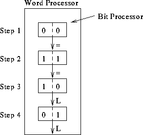
Compare, notify.
Assume we have k-bit numbers. Run time?
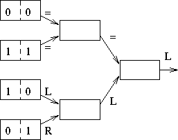
Compare, notify.
Run time?
Notes:
- Why not use a height 1 tree?
- Fan-in and fan-out in circuits.
Tom Kelliher, CS 315
Feb. 3, 1999
Read Sections 1.1.4, 1.1.5.
Sorting in the Bit Model.
Lower bound counterexample, properties of fixed-connection networks.

Compare, notify.
Assume we have k-bit numbers. Run time?

Compare, notify.
Run time?
Notes:
What do they look like?
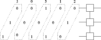
Five in, four out.
A lot of parallel work. Systolic computation.

Running time?
 steps on an
  -processor machine. Which algorithm is more
efficient?
Assume that the cost of running a P-processor machine for T steps is
 , where
  and
and  are constants and P = M or
 . For what values of
  and
and  is the first algorithm
cheaper to run? For what values of
  and
and  is the second
algorithm cheaper to run?
 steps
on an
  -processor machine. Which algorithm will run faster on an
N-processor machine? (Hint: Your answer depends on the relative sizes of
M and N, and you will need to use the fact that an N-processor
machine can simulate a P-processor machine with slowdown
  .)
.)
The following are tools we can sometimes use to characterize a problem-solving network and, hence, understand its failings.
Assume the bit model, so we have an  sorting network in the
following.
What is the I/O bandwidth of the sorting network? This makes sorting
 .
.
What is the diameter of the sorting graph?
Can we construct a sorting problem that will force the two most distant cells to communicate?
What's the lower bound from this perspective?
What is the bisection width of the sorting graph?
Can we construct a sorting problem that will force all the data to cross this boundary?
What's the lower bound from this perspective?